Chapter 13 Introduction to K-Means Clustering
When diving into the world of unsupervised learning, one of the most straightforward yet powerful algorithms you’ll encounter is k-means clustering. It’s like sorting your socks by color and size without knowing how many pairs you have in the first place. K-means helps to organize data into clusters that exhibit similar characteristics, making it a fantastic tool for pattern discovery and data segmentation.
13.1 Why K-Means Clustering?
K-means clustering is used extensively across different fields, from market segmentation and data compression to pattern recognition and image analysis. It groups data points into a predefined number of clusters (k) based on their features, minimizing the variance within each cluster. The result? A clear, concise grouping of data points that can reveal patterns and insights which might not be immediately obvious.
13.1.1 How Does K-Means Work?
The process is beautifully simple:
- Select k points as the initial centroids randomly.
- Assign each data point to the nearest centroid.
- Recompute the centroid of each cluster by taking the mean of all points assigned to that cluster.
- Repeat the assignment and centroid computation steps until the centroids no longer move significantly, which indicates that the clusters are stable and the algorithm has converged.
This method partitions the dataset into Voronoi cells, which are essentially the k regions we aim to discover, where each point is closer to its own cluster centroid than to others.
13.2 Practical Example: K-Means on the Iris Dataset
Let’s put theory into practice with the Iris dataset, where we’ll attempt to cluster the flowers based solely on their petal and sepal measurements.
# Load necessary libraries
library(stats)

# Load the iris dataset
data(iris)

# Use only the petal and sepal measurements
iris_data <- iris[, 1:4]

# Set a seed for reproducibility
set.seed(123)

# Perform k-means clustering with 3 clusters (as we expect 3 species)
km_result <- kmeans(iris_data, centers = 3, nstart = 25)

# View the results
print(km_result$centers)
## Sepal.Length Sepal.Width Petal.Length Petal.Width
## 1 5.006000 3.428000 1.462000 0.246000
## 2 5.901613 2.748387 4.393548 1.433871
## 3 6.850000 3.073684 5.742105 2.07105313.2.1 Visualizing K-Means Clustering
To see our clustering in action, let’s plot the clusters along with the centroids:
library(ggplot2)

# Create a data frame with the cluster assignments
iris_clusters <- data.frame(iris_data, Cluster = factor(km_result$cluster))

# Plotting
ggplot(iris_clusters, aes(Petal.Length, Petal.Width, color = Cluster)) +
  geom_point(alpha = 0.5) +
  geom_point(data = data.frame(km_result$centers), aes(x = Petal.Length, y = Petal.Width),
             colour = 'red', size = 5, shape = 17) +
  ggtitle("K-Means Clustering of the Iris Dataset") +
  theme_minimal()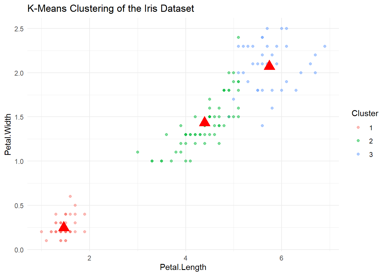
This plot will shows how the algorithm groups the flowers into clusters, with red points marking the centroids. Each cluster corresponds to groups of flowers that share similar petal and sepal dimensions. Based on these two dimentions we can see that these flowers are nicely clustered!
13.3 The Math of K-Means Clustering: Getting the Grouping Right
At its core, k-means clustering is all about grouping things neatly and effectively. Think of it as organizing a jumbled set of books into neatly labeled categories on a shelf. In k-means, our “books” are data points, and the “categories” are clusters. The goal? To make sure each book finds its perfect spot where it fits the best.
13.3.1 The Math Behind Perfect Grouping
Let’s break down the magic formula that k-means uses to achieve this tidy arrangement:
\[ \text{arg } \underset{\mathcal{Z}, A}{\text{ min }}\sum_{i=1}^{N}||x_i-z_{A(x_i)}||^2 \]
Here’s what this equation is telling us: - Every data point \(x_i\) is trying to find its closest cluster center \(z\) from a set of possible centers \(\mathcal{Z}\). - \(A(x_i)\) is the rule that decides which cluster center is the best match for \(x_i\). - The double bars \(||x_i - z_{A(x_i)}||^2\) represent the “distance” each book (data point) is from its designated spot on the shelf (cluster center). Our goal is to minimize this distance so that every book is as close as possible to its ideal location.
13.3.2 How K-Means Tidies Up
- Starting Lineup: First, we pick a starting lineup by randomly selecting a few cluster centers.
- Finding Friends: Each data point looks around, finds the nearest cluster center, and joins that group.
- Regrouping: Once everyone has picked a spot, each cluster center recalculates its position based on the average location of all its new friends.
- Repeat: This process of finding friends and regrouping continues until everyone is settled and the centers don’t need to move anymore.
13.3.3 Why Do We Care?
Understanding this objective function is like knowing the rules of the game. It helps us see why k-means makes certain decisions: grouping data points based on similarity, adjusting cluster centers, and iteratively refining groups. It’s about creating clusters that are as tight-knit and distinct as possible, which is essential when we’re trying to uncover hidden patterns in our data.
This clustering isn’t just about neatness, it’s about making sense of the chaos. By minimizing the “distances” or differences within groups, k-means helps ensure that each cluster is a clear, distinct category that tells us something meaningful about the data. It’s a powerful way to turn raw data into insights that can inform real-world decisions.