Chapter 6 Introduction to Linear Regression

Linear regression might sound complex, but let’s break it down to something as simple as fitting a line through a set of points, just like you might have done in middle school. Remember the equation \(y = mx + b\)? We’re going to start there. Remember m is the slope, and b is the intercept? Well, all regression does is solve for that using your data!

6.1 The Concept

In statistical terms, this line equation becomes \(y = \alpha + \beta \times x + \epsilon\), where:

\(\alpha\) (alpha) is the y-intercept,
\(\beta\) (beta) is the slope of the line,
\(\epsilon\) (epsilon) or the error is the difference between the predicted values and the actual values.

6.1.1 Visualizing Simple Attempts

Let’s imagine a “Dan Estimator” and “Steve Estimator” are trying to draw a line through some data points. Both are pretty bad at it. Their lines don’t really capture the trend of the data.

# Simulate some data
set.seed(42)
x <- 1:100
y <- 2*x + rnorm(100, mean=0, sd=20)  # true line: y = 2x + noise
plot(x, y, main = "Fitting Lines: Dan vs. Steve", xlab = "X", ylab = "Y", pch = 19)

# Dan's and Steve's poor attempts
lines(x, 4*x - 40, col = "red")  # Dan's line
lines(x, .5*x + 30, col = "blue")  # Steve's line
legend("topright", legend=c("Dan", "Steve"), col=c("red", "blue"), lty=1, cex=0.8)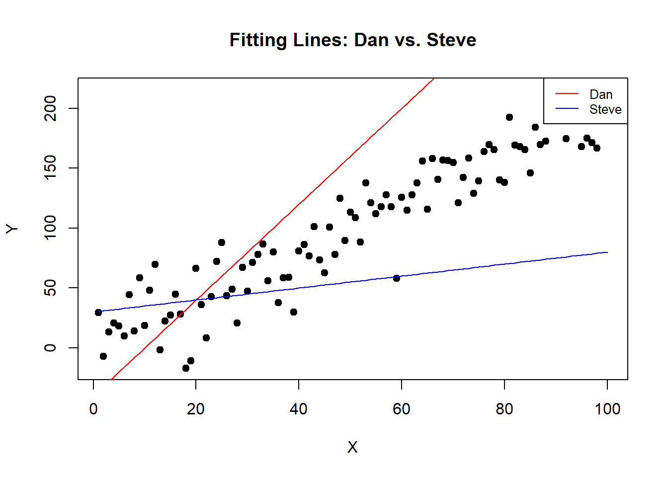

6.1.2 Finding the Best Fit

Now, while Dan and Steve’s attempts are entertaining, they’re obviously not ideal. Maybe we want an estimator that draws a line right through the middle of these points? One that minimizes the distance from all points to the line itself. How can we ensure it’s the best fit?

6.1.2.1 Introducing Least Squares

We want to fit a line through the middle one where we minimize the distance from the line to the points on average. In otherwords we aim to minimize the sum of the squared distances (squared errors) from the data points to the regression line. This method is called “least squares.”

set.seed(42)
x <- 1:100
y <- 2*x + rnorm(100, mean=0, sd=20)

# Fitting a regression line
fit <- lm(y ~ x)

# true line: y = 2x + noise
plot(x, y, main = "Fitting Lines: Dan vs. Steve vs. Least Squares", xlab = "X", ylab = "Y", pch = 19)

# Dan's and Steve's poor attempts
lines(x, 4*x - 40, col = "red")  # Dan's line
lines(x, 0.5*x + 30, col = "blue")  # Steve's line
abline(fit, col="black")  # adding the least squares line

# Adding residuals for the least squares line
predicted_values <- predict(fit)
for (i in 1:length(x)) {
    lines(c(x[i], x[i]), c(y[i], predicted_values[i]), col="black")
}

legend("topright", legend=c("Dan", "Steve", "Least Squares"), col=c("red", "blue", "black"), lty=1, cex=0.8)


# Add a legend for the residuals
legend("bottomright", legend=c("Residuals"), col=c("black"), lty=1, cex=0.8)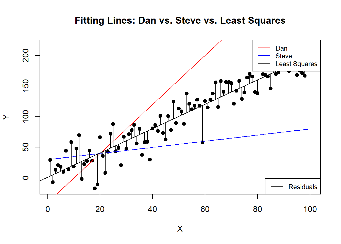

Here we can see that the Least Squares line goes right through the middle and on average the distance from the line, the “residuals” are about the same on top as they are on the bottom.

6.2 Understanding the Interpretation

The regression equation can be written as: \[ y = \alpha + \beta \times x + error\] where \(\hat{\alpha}\) and \(\hat{\beta}\) are estimates of the intercept and slope, determined by the least squares method.

So all you have to do to understand the relationship x has to y is to plug in the numbers you get from the model!

So if \(\beta = 2\). That means a 1 unit increase in \(x = 1\) results in a \(2 \times x\) increase in y! It is that easy.

Want to know what y is on average controlling for your variables?

Let’s take the mtcars dataset, which contains the variables: mpg, Weight (1000 lbs), Displacement (cu.in.), Horsepower, and Number of cylinders. We want to know if we can predict mpg based on these factors.

# Load the dataset
data(mtcars)

head(mtcars)

##                    mpg cyl disp  hp drat    wt  qsec vs am gear carb
## Mazda RX4         21.0   6  160 110 3.90 2.620 16.46  0  1    4    4
## Mazda RX4 Wag     21.0   6  160 110 3.90 2.875 17.02  0  1    4    4
## Datsun 710        22.8   4  108  93 3.85 2.320 18.61  1  1    4    1
## Hornet 4 Drive    21.4   6  258 110 3.08 3.215 19.44  1  0    3    1
## Hornet Sportabout 18.7   8  360 175 3.15 3.440 17.02  0  0    3    2
## Valiant           18.1   6  225 105 2.76 3.460 20.22  1  0    3    1

There you go! Its just like an excel spreadsheet if you never encountered a dataset in R before.

# Load the dataset
data(mtcars)

cars <- lm(mpg ~ wt + disp + hp + cyl, data = mtcars)
summary(cars)

## 
## Call:
## lm(formula = mpg ~ wt + disp + hp + cyl, data = mtcars)
## 
## Residuals:
##     Min      1Q  Median      3Q     Max 
## -4.0562 -1.4636 -0.4281  1.2854  5.8269 
## 
## Coefficients:
##             Estimate Std. Error t value Pr(>|t|)    
## (Intercept) 40.82854    2.75747  14.807 1.76e-14 ***
## wt          -3.85390    1.01547  -3.795 0.000759 ***
## disp         0.01160    0.01173   0.989 0.331386    
## hp          -0.02054    0.01215  -1.691 0.102379    
## cyl         -1.29332    0.65588  -1.972 0.058947 .  
## ---
## Signif. codes:  0 '***' 0.001 '**' 0.01 '*' 0.05 '.' 0.1 ' ' 1
## 
## Residual standard error: 2.513 on 27 degrees of freedom
## Multiple R-squared:  0.8486, Adjusted R-squared:  0.8262 
## F-statistic: 37.84 on 4 and 27 DF,  p-value: 1.061e-10

Here are the results of the model! the Summary function provides a lot of information. For our estimates, we want the Estimate column. The remaining columns are for measuring if the effect is significant or not. The information at the bottom tells us goodness of our fit.

Let’s go back top that Estimate column. These are our \(\beta\)s. So we have this formula

\[ \operatorname{mpg} = \alpha + \beta_{1}(\operatorname{wt}) + \beta_{2}(\operatorname{disp}) + \beta_{3}(\operatorname{hp}) + \beta_{4}(\operatorname{cyl}) + \epsilon \] When you plug in the betas you get:

\[ \operatorname{\widehat{mpg}} = 40.83 - 3.85(\operatorname{wt}) + 0.01(\operatorname{disp}) - 0.02(\operatorname{hp}) - 1.29(\operatorname{cyl}) \] Which means all you have to do is plug the numbers for the Xs.

Let’s say we want to know the average mpg of a car that weights 4,000 lbs, has 145 Horse Power, 150 cubic inch displacement engine, and 4 cylinders.

\[ \operatorname{\widehat{mpg}} = 40.83 - 3.85(\operatorname{4}) + 0.01(\operatorname{150}) - 0.02(\operatorname{145}) - 1.29(\operatorname{4}) \] which equals 18.87 mpg! That seems reasonable for a car a few ago (when the cars in this dataset are from).

6.2.1 Going a Step Further: Linear Algebra

For those interested in the mathematical details, the coefficients \(\beta\) can also be estimated using linear algebra. This is expressed as: \[ \beta = (X^TX)^{-1}X^TY \] where \(X\) is the matrix of input values, and \(Y\) is the vector of output values. This formula provides the least squares estimates of the coefficients.

6.2.1.1 Load and Prepare Data

First, let’s load the data and prepare the matrices.

# Prepare the data matrix X (with intercept) and response vector Y
X <- as.matrix(cbind(Intercept = 1, `Weight (1000 lbs)` = mtcars$wt, `Displacement (cu.in.)` = mtcars$disp, `Horsepower` = mtcars$hp, `Number of cylinders` = mtcars$cyl))  # Adding an intercept
Y <- mtcars$mpg

# Display the first few rows of X and Y
head(X)

##      Intercept Weight (1000 lbs) Displacement (cu.in.) Horsepower Number of cylinders
## [1,]         1             2.620                   160        110                   6
## [2,]         1             2.875                   160        110                   6
## [3,]         1             2.320                   108         93                   4
## [4,]         1             3.215                   258        110                   6
## [5,]         1             3.440                   360        175                   8
## [6,]         1             3.460                   225        105                   6

head(Y)

## [1] 21.0 21.0 22.8 21.4 18.7 18.1

6.2.1.2 Apply the Linear Algebra Formula for Beta

Now, we apply the linear algebra formula to compute the coefficients. The formula \(\beta = (X^TX)^{-1}X^TY\) will give us the estimates for the intercept and the coefficient for mpg.

# Compute (X'X)^(-1)
XTX_inv <- solve(t(X) %*% X)

# Compute beta = (X'X)^(-1)X'Y
beta <- XTX_inv %*% t(X) %*% Y

# Print the estimated coefficients
beta

##                              [,1]
## Intercept             40.82853674
## Weight (1000 lbs)     -3.85390352
## Displacement (cu.in.)  0.01159924
## Horsepower            -0.02053838
## Number of cylinders   -1.29331972

This isn’t as pretty but check that out! We can see that increasing the weight of the car by 1000 lbs results in a 3.85 mpg reduction holding the rest of the variables equal. the Horsepower and Displacement (cu.in.) show small effects, adding a cylinder to the engine reduces mpg by 1.29. The intercept here makes little sense because that would mean cars get around 41 mpg if they had 0 weight, Horsepower, etc.

Math works! In all seriousness though computers are much faster at solving \(\beta = (X^TX)^{-1}X^TY\) than running that function, so if you are computing many \(\beta\)s at once, it can come in handy.

6.3 Assumptions of Linear Regression

To effectively use linear regression, it’s essential to understand its underlying assumptions. If these assumptions are violated, the results might not be reliable. Here are the key assumptions:

Linearity: The relationship between the predictors and the dependent variable is linear.
Independence: Observations are independent of each other.
Homoscedasticity: The variance of residual is the same for any value of the input variables.
Normality: For any fixed value of the predictors, the dependent variable is normally distributed.

Addressing these assumptions ensures the validity of the regression results. When these assumptions are not met, modifications and more advanced techniques might be necessary.

6.4 Extending Linear Regression

As powerful as linear regression is, it sometimes needs to be adjusted or extended to handle more complex data characteristics. Here are a few notable extensions:

6.4.1 Spatial Regression

When dealing with geographical or spatial data, traditional regression might not suffice because observations in close proximity might be correlated, violating the independence assumption. Spatial regression models account for this correlation, offering more precise insights for geographical data analysis.

6.4.2 Robust Estimation

Robust estimators are a broad class of estimators that generalize the method of least squares. They are particularly useful when dealing with outliers or heavy-tailed distributions, as they provide robustness against violations of the normality assumption.

6.4.3 Robust Standard Errors

Robust standard errors are an adjustment to standard errors in regression analysis that provide a safeguard against violations of both the homoscedasticity and independence assumptions. They are essential for drawing reliable inference when these assumptions are challenged.

6.4.4 Handling Serial Autocorrelation in Time Series Data

When dealing with time series data, one common challenge is serial autocorrelation—where residuals at one point in time are correlated with residuals at a previous time. This correlation can invalidate standard regression inferences because it breaches the assumption that the error terms are independent. To address this, methods like ARIMA models or adjustments such as Newey-West standard errors can be used to correct for the autocorrelation, ensuring the integrity of the regression analysis.

By incorporating these extensions into your analytical toolkit, you can tackle a broader range of data characteristics and draw more reliable conclusions from your statistical models.