Chapter 14 Introduction to Machine Learning: Random Forests
As we venture into the realm of machine learning, one of the most robust and widely-used algorithms we encounter is the Random Forest. It builds on the simplicity of decision trees and enhances their effectiveness.
14.1 Why Random Forests?
Random Forests operate by constructing a multitude of decision trees at training time and outputting the class that is the mode of the classes (classification) or mean prediction (regression) of the individual trees. They are known for their high accuracy, ability to run on large datasets, and their capability to handle both numerical and categorical data.
14.2 Understanding Random Forests by Starting with a Single Tree
How do you describe a forest to someone who has never seen a tree? Similarly, to understand random forests, it helps to start by understanding individual trees. A random forest is essentially a collection of decision trees where each tree contributes to the final outcome. Let’s dive into this by looking at a basic decision tree model.
A decision tree is trained using a process called recursive binary splitting. This is a greedy algorithm that divides the space into regions by making splits at values of the input features that result in the most significant improvement in homogeneity of the target variable.
14.2.1 How are Splits Determined?
During the training of a decision tree, the best split at each node is chosen by selecting the split that maximizes the decrease in impurity from the parent node to the child nodes. Several metrics can be used to measure impurity, including Gini impurity, entropy, and classification error in classification tasks, or variance reduction in regression.
The algorithm:
- Considers every feature and every possible value of each feature as a candidate split.
- Calculates the impurity reduction (or information gain) that would result from splitting on the candidate.
- Selects the split that results in the highest gain.
- Recursively applies this process to the resulting subregions until a stopping criterion is met (e.g., a maximum tree depth, minimum number of samples in a leaf).
This greedy approach ensures that the model is as accurate as possible at each step, given the previous splits, but it doesn’t guarantee a globally optimal tree. This is where the power of random forests comes in, by building many trees, each based on a random subset of features and samples, and averaging their predictions, the ensemble model counters the variance and potential overfitting of individual trees.
14.2.2 Example: Decision Tree with the Iris Dataset
Now that we have a foundational understanding of how decision trees are trained, let’s apply this knowledge by training a model using the Iris dataset.
# Load necessary libraries
library(rpart)
library(rpart.plot)

# Split the data into training and test sets
set.seed(123)  # for reproducibility
train_index <- sample(1:nrow(iris), size = 0.7 * nrow(iris))
train <- iris[train_index, ]
test <- iris[-train_index, ]
Now, let’s train a decision tree model on the training set. We’ll use the model to predict the species of iris based on its features (sepal length, sepal width, petal length, and petal width):
14.2.3 Visualizing the Decision Tree
With our model trained, we can visualize it to better understand how decisions are made:
14.2.4 Decision Tree Insights
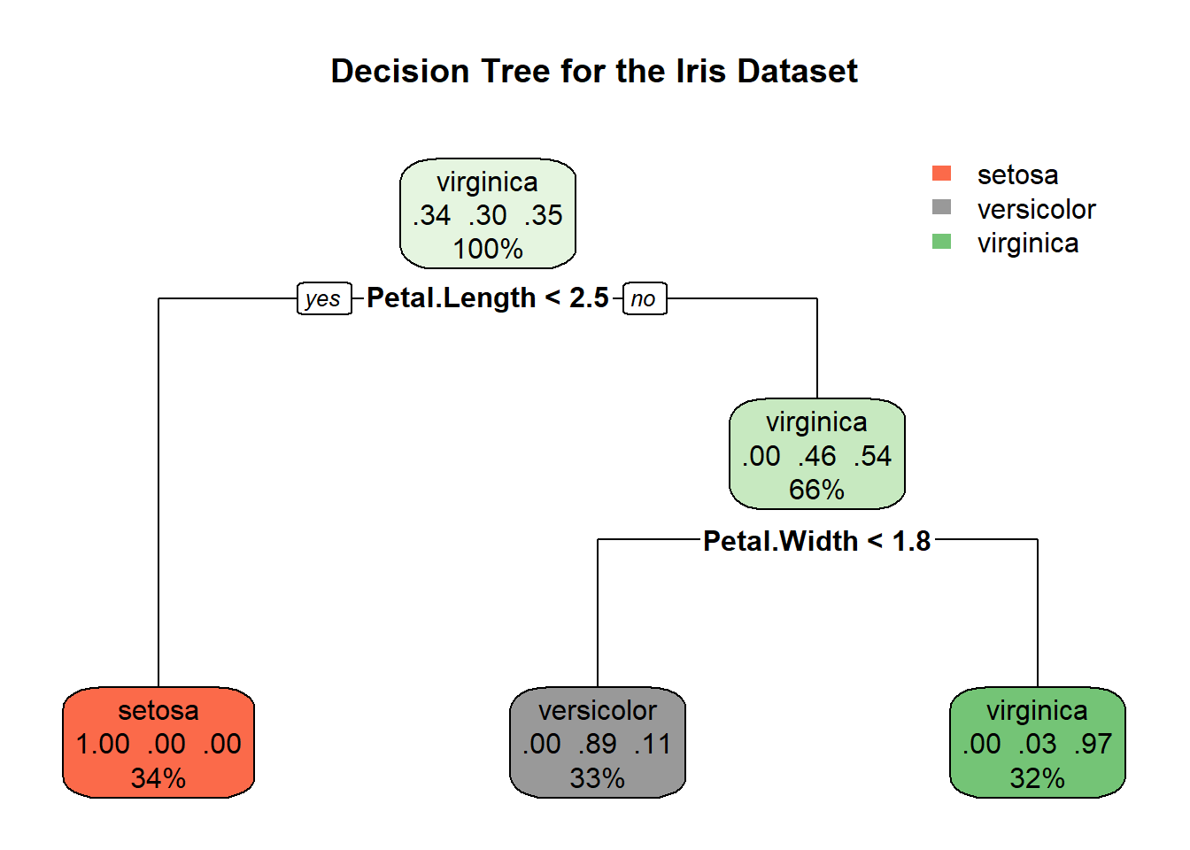
The decision tree visualized above provides a clear pathway of how the model determines the species of iris based on petal and sepal measurements. Let’s break down the key elements:
Root Node: The decision-making starts at the root, where the first split is based on petal length. If the petal length is less than or equal to 2.5 cm, the tree predicts the species to be Setosa. This is visible in the leftmost leaf, indicating a 100% probability for Setosa with 34% of the sample falling into this category.
Intermediate Nodes and Splits: For observations where petal length exceeds 2.5 cm, further splits occur:
- The next decision node uses petal width, splitting at 1.8 cm. Observations with petal width less than or equal to 1.8 cm lead to another node, which finally splits based on sepal width.
Leaves (Final Decisions):
- Left Leaf: As noted, all observations with petal length ≤ 2.5 cm are classified as Setosa.
- Middle Leaves: These represent observations with longer petal lengths but smaller petal widths (≤ 1.8 cm). These leaves predict Versicolor or Virginica, depending on additional criteria like sepal width.
- Right Leaf: Observations with petal length > 2.5 cm and petal width > 1.8 cm are mostly classified as Virginica (probability of 97%), with a small percentage predicted as Versicolor.
14.3 Step-by-Step Example with Random Forests
A single decision tree is often a “shallow learner” good at learning simple structures. A random forest combines many such trees to create a “strong learner” that can model complex relationships within the data.
Let’s use the randomForest package in R to demonstrate how to use random forests for a classification problem.
14.3.1 Setting Up the Problem
Let’s use iris dataset again. We’ll predict the species of iris plants based on four features: sepal length, sepal width, petal length, and petal width.
# Load necessary library
library(randomForest)

# Load the iris dataset
data(iris)

# Fit a random forest model
rf_model <- randomForest(Species ~ ., data = iris, ntree = 100)
print(rf_model)
##
## Call:
## randomForest(formula = Species ~ ., data = iris, ntree = 100)
## Type of random forest: classification
## Number of trees: 100
## No. of variables tried at each split: 2
##
## OOB estimate of error rate: 4.67%
## Confusion matrix:
## setosa versicolor virginica class.error
## setosa 50 0 0 0.00
## versicolor 0 47 3 0.06
## virginica 0 4 46 0.0814.3.2 Visualizing the Ensemble Effect
While we cannot visualize all trees at once, plotting the error rate as more trees are added can demonstrate the ensemble effect.
# Plot error rate versus number of trees
plot(rf_model$err.rate[,1], type = "l", col = "red")
title("Error Rate of Random Forest Over Trees")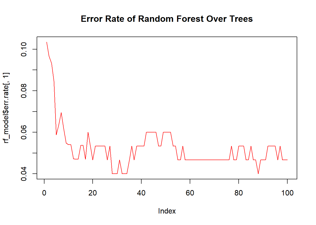
This plot typically shows that as more trees are added, the error rate of the random forest stabilizes, demonstrating the power of combining many models.
14.3.3 Using the Model
Let’s demonstrate using the trained model to predict the species of a new iris flower.
# New flower data
new_flower <- data.frame(Sepal.Length = 5.0, Sepal.Width = 3.5, Petal.Length = 1.4, Petal.Width = 0.2)

# Predict the species
predict(rf_model, new_flower)
## 1
## setosa
## Levels: setosa versicolor virginica