Chapter 12 Logistic Regression: Going Beyond Linear Regression
While linear regression is suited for continuous outcomes, what do we do when our dependent variable is binary, like “yes” or “no,” “success” or “failure”? This is where logistic regression comes into play.
12.1 Why Use Logistic Regression?
Logistic regression is used when the dependent variable is categorical and binary. It allows us to estimate the probability that a given input belongs to a certain category, based on the logistic function.
12.2 The Logistic Function
The logistic function, also known as the sigmoid function, ensures that the output of the regression model is always between 0 and 1, making it interpretable as a probability. The equation for logistic regression is:
\[ p(x) = \frac{1}{1 + e^{-(\beta_0 + \beta_1x_1 + \beta_2x_2 + \ldots + \beta_nx_n)}} \]
where \(p(x)\) represents the probability that the dependent variable equals 1 given the predictors \(x_1, x_2, \ldots, x_n\).
12.2.1 Visualizing the Sigmoid Function
The beauty of the logistic (sigmoid) function lies in its ability to squash the entire range of real numbers into a bounded interval of [0, 1], making it perfect for probability modeling. Let’s plot this function to see how changes in the input (from negative to positive values) smoothly transition the output from 0 to 1. This transition exemplifies how logistic regression manages probability estimations.
# Generate values for the input
x_values <- seq(-10, 10, length.out = 100)

# Calculate the sigmoid function values
sigmoid_values <- 1 / (1 + exp(-x_values))

# Create the plot
plot(x_values, sigmoid_values, type = 'l', col = 'blue', lwd = 2,
     main = "Visualization of the Sigmoid Function",
     xlab = "Input Value (x)", ylab = "Sigmoid Output (p(x))",
     ylim = c(0, 1))

# Add lines to indicate the midpoint transition
abline(h = 0.5, v = 0, col = 'black', lty = 2)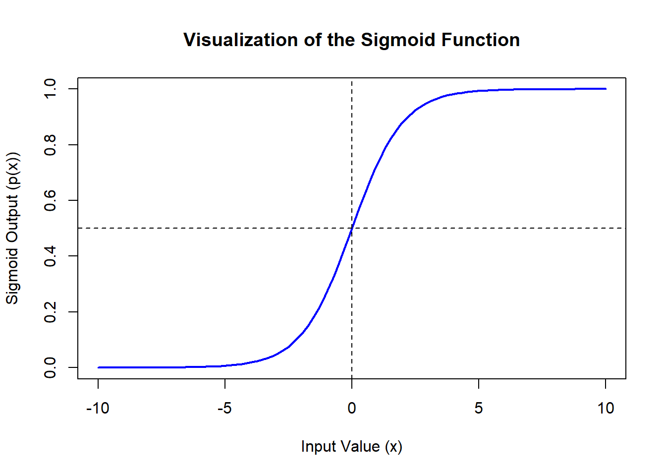
12.2.2 What Does This Plot Show?
- Horizontal Line (black, Dashed): This line at \(p(x) = 0.5\) marks the decision threshold in logistic regression. Values above this line indicate a probability greater than 50%, typically classified as a “success” or “1”.
- Vertical Line (black, Dashed): This line at \(x = 0\) shows where the input to the function is zero. It’s the point of symmetry for the sigmoid function, highlighting the balance between the probabilities.
This plot beautifully illustrates the gradual, smooth transition of probabilities, characteristic of the logistic function. By moving from left to right along the x-axis, we can observe how increasingly positive values push the probability closer to 1, which is precisely how logistic regression models the probability of success based on various predictors.
12.3 Demonstration in R
Let’s demonstrate logistic regression by considering a dataset where we predict whether a student passes (1) or fails (0) based on their hours of study.
12.3.2 Fitting a Logistic Regression Model
# Fitting the model
logit_model <- glm(pass ~ hours_studied, family = binomial(link = "logit"), data = student_data)

# Summarizing the model
summary(logit_model)
##
## Call:
## glm(formula = pass ~ hours_studied, family = binomial(link = "logit"),
## data = student_data)
##
## Coefficients:
## Estimate Std. Error z value Pr(>|z|)
## (Intercept) -4.4802 0.9177 -4.882 1.05e-06 ***
## hours_studied 0.9059 0.1693 5.351 8.75e-08 ***
## ---
## Signif. codes: 0 '***' 0.001 '**' 0.01 '*' 0.05 '.' 0.1 ' ' 1
##
## (Dispersion parameter for binomial family taken to be 1)
##
## Null deviance: 137.989 on 99 degrees of freedom
## Residual deviance: 66.504 on 98 degrees of freedom
## AIC: 70.504
##
## Number of Fisher Scoring iterations: 612.3.3 Visualizing the Results
# Plotting the fitted probabilities
plot(student_data$hours_studied, student_data$pass, col = ifelse(student_data$pass == 1, "green", "red"), pch = 19, main = "Probability of Passing based on Hours Studied")
curve(predict(logit_model, data.frame(hours_studied = x), type = "response"), add = TRUE)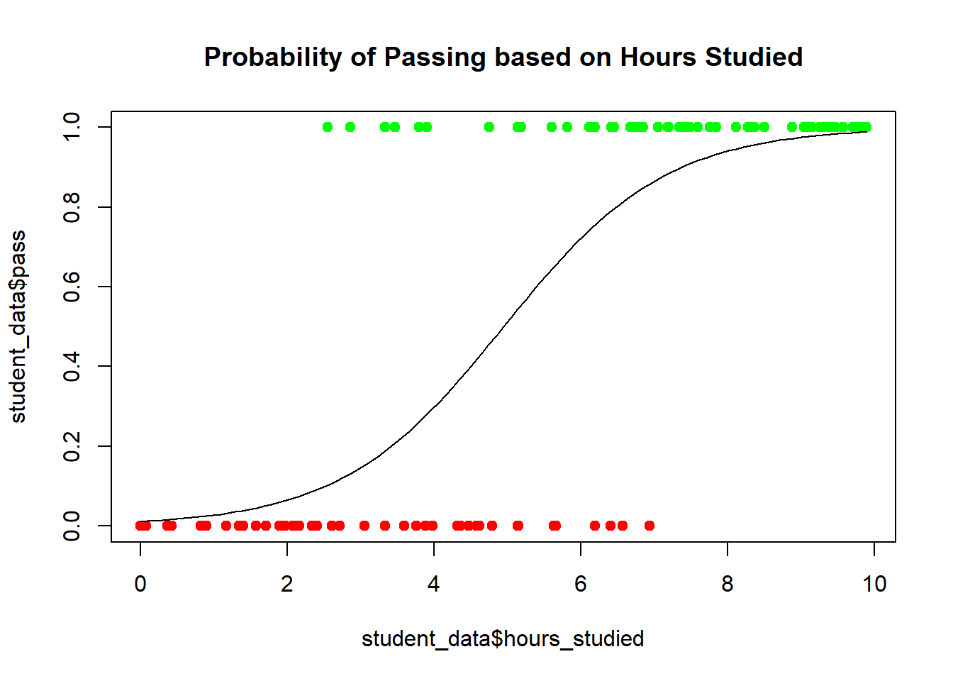
This plot shows the probability of a student passing based on their hours of study, with the logistic regression model providing a smooth probability curve.